Reconstruction Error

Reconstruction Error is the fourth project in this portfolio. It is a set of five pieces, presented in an EP format.

There is also a git repository that contains all of the Python code and Max patches that were created and used as part of this project. This repository can be found here: /Projects/Reconstruction Error/Supporting Code.

Motivations and Influences

In the previous three projects, I explored a number of techniques, approaches and workflows for computer-aided composition with content-aware programs. Each of these projects was motivated by a combination of factors both musical and extra-musical, such as opportunities to compose for visiting artists or the need to respond to immediate influences in my creative coding practice and musical listening. Reflecting on the previous projects up to this point, the most successful and fluid workflow evolved in Stitch/Strata. Despite being a difficult compositional process that involved many failed attempts to reach the finished state of the piece, using the computer to sieve through a corpus of sounds and offer up generated sections of material and sound was an expressive workflow in which agency was balanced between me and the computer. I decided to move forward with this model in mind and aimed to create a piece by using the computer in a similar fashion.

Databending

Amongst this reflection on my practice up to this point, I had been listening to artists such as Alva Noto, Autechre, Opiate and Ryoji Ikeda. Their work draws on hyper-digital, surgical and sometimes ultra-minimalist sonic materials associated with post-digital aesthetics. The raw digital sounds found in this sphere of music have always been appealing to me, and an integral part of my compositional vocabulary and aesthetic. Stitch/Strata, while using entirely organically generated vocal sounds, engenders a strong machine and digital aesthetic by the way that sounds are arranged and processed. Similarly, the signal-processing modules in Refracted Touch at times conceal the “human” elements of Daryl Buckley’s playing, and transform sound materials that he generates into synthetically altered versions of them.

I was also becoming interested in databending, a process in which raw data is used to construct visual and sonic materials. This can be achieved in several ways, and the nature of this process can itself have a significant impact on the results. Several existing tools facilitate databending, either intentionally or through divergent and unintended application. Examples include SoundHack, which allows one to convert any file on a computer into a valid WAVE audio file; Audacity, which supports the reading of raw bytes as audio data; and PhotoShop, which can open non-image files as if they were images.

A number of artists have experimented with databending in their work and this has guided my research into this digital practice. Nick Briz explores various “attacks” on video data to degrade and produce distortions in Binary Self-Portraits (2008) (see VIDEO 4.4.1). Another of Briz’s works, From The Group Up In Order, Embrace (2007) (see VIDEO 4.4.2), explores the creation of visual material through the interface of the binary code that represents itself. Briz states that:

Unitxt Code (Data to AIFF) (2008) (see VIDEO 4.4.3) by Alva Noto, although not explicitly stated in liner notes or interviews, likely uses data converted to audio (as suggested by the name) for the core compositional material of that work. The harsh and degraded noise-based sounds which are heard in this work are commonly produced when converting text files into audio. Datamatics (2006) (see VIDEO 4.4.4), by Ryoji Ikeda incorporates raw data as source material which drives both the visual and audio of this installation work. Pimmon’s album Electronic Tax Return (2007) (see VIDEO 4.4.5) has several works based on synthesising sound by converting dynamic-link libraries (.dll files) into files for playback and manipulation.

These works of sound art and composition were part of my exposure and research into databending. In particular, Michael Chinen’s practical experiments were instrumental in drawing me into a “hacker’s” approach through the creation of custom software. Chinen’s work almost exclusively focuses on the sonification of data from random-access memory (RAM). One of these works, FuckingAudacity, is a fork of the popular audio application Audacity. The sound output from this fork is generated by using the memory state of the program as audio data for the system output buffer at regular intervals. Interactions with the user interface and user-driven processes such as importing files or enabling effects themselves become ways of manipulating the sound output. VIDEO 4.4.6 is a demonstration of Chinen playing with the program.

FuckingWebBrowser (see VIDEO 4.4.7) follows suit from its Audacity counterpart. The application presents as a standard web browser. However, the memory state of the program is used to generate audio data which is then played back as the user interacts with the software. Navigating to or from a website or interacting with a page generates sounds in unpredictable ways. Even doing nothing at times reveals the program’s hidden internal workings as sounds. Making HTTP requests, polling for data, or caching files in the background results in sounds that are not tightly coupled to the user’s interaction with the application.

The logical conclusion to this suite of custom databending applications is one that can be attached to any program. lstn performs this function, and can observe and sonify the opcodes, call stack and active memory of any program on the computer. VIDEO 4.4.8 is a demonstration of this in practice, where it is attached to several different running programs in real-time.

Employing the Computer to Structure a Corpus

Coming into contact with Chinen’s work was influential because there is a mixture of predictable and unpredictable sonic behaviours exhibited by the computer through his various databending programs. The overarching character of the generated sound is digital, harsh and noise-based, but occasionally these processes produce silence as well as sounds that are fragile and delicate. This notion of there being “needles in the haystack” was a tension that I wanted to explore myself. How could I generate a large body of material and search for the “needles”? Part of my motivation for this project was to create a set of conditions in which I could explore this realm, and mediate that investigation using the computer as part of the compositional process.

As part of my preliminary research in this area, I came into contact with the outputs of the Fluid Corpus Manipulation (FluCoMa) project. I had up to this point been loosely involved with some of their research activities and privy to internal workshops with their commissioned composers as a helper. As such, I was able to view a pre-release video demonstration for FluidCorpusMap (see VIDEO 4.4.9). Neither the paper (Roma et al., 2019) or the source code for this program were released at the time, which hindered my ability to understand the software in a detailed way. However, the video broadly points out that it is using mel-cepstrum frequency coefficients (MFCCs), audio descriptor analysis, statistical summaries and a dimension reduction algorithm to create a two-dimensional latent space for exploration and navigation. I found two aspects of this process fascinating. Firstly, the global visual aspect of the dimension reduction was novel and possessed unique characteristics depending on the algorithm. For me, each layout was evocative, in that the computer seemed to be creating its own machine-like understanding of the corpus. Secondly, the local distribution of samples was perceptually smooth and coherent. Movements between adjacent points in the demonstration returned texturally similar sounds. Even aspects such as morphology seemed to be captured (this can be seen around 1:19, where sounds with upwards glissandi are grouped together), giving the sense that the computer could listen to texture and morphology. This, to me, was far more sophisticated than my previous experiments using instantaneous statistical summaries, such as in Stitch/Strata.

In my previous projects, searching for sounds within collections has been of interest to me, albeit using different technologies and analytical approaches than FluidCorpusMap. For example, the compositional building blocks of Stitch/Strata were produced by selecting samples from a corpus by audio descriptor query. Similarly, the simulated annealing algorithm searches through a complex latent space in which a single parametric input is coupled to an audio descriptor output. Both of these approaches are based on calculating audio features with descriptors and then using those features as constraints or selection criteria in order to filter samples from a corpus.

FluidCorpusMap presents its own solution to such a problem, positioning the interactive relationship between user and computer as one where the human interprets the machine’s portrayal and decomposition of the latent space. Rather than having to find a suitable way of representing the relationship between sounds through several audio descriptors, the dimension reduction process attempts to figure this out automatically and then offers it back to the user in a compressed and visual form. To me, this seemed like it might be more fruitful in navigating speculatively through unknown sound collections and then having the computer structure my engagement with sonic materials. With that in mind, I moved forward into the practical part of this project. This is discussed in [4.4.2 Initial Technological Experimentation].

Initial Technological Experimentation

This section outlines the technology and development of software situated at the start of the composition process. It outlines five key stages of a processing pipeline, beginning with the generation of a corpus using databending techniques.

Generation

I began composing Reconstruction Error by generating a corpus of materials using databending techniques. Ultimately, I wanted to create a large corpus of sounds that I would initially have little understanding of. From that point, I intended to use machine listening to structure my investigation of those materials, formulating the piece as a hybrid of my own and the computer’s agency.

I began databending by modifying the code of Alex Harker’s ibuffer~ Max object so that it could load any file, not just those intended to store audio data for playback. Reading audio files such as WAVE and AIFF typically involves parsing a section of bytes at the start of the file, the “header”, which tells the program how to interpret the structure of another chunk of data which is the audio itself. My forked version of ibuffer~ operated by adding a new method to the object, readraw which could read a file without looking for the header, and instead assumed that all the data in the file was 8-bit encoded 44.1kHz sample-rate mono audio. Some of the conversions from this process can be found in AUDIO 4.4.2. Note that these samples have been reduced in volume by 90% because the originals were excessively loud.

Using the fork of ibuffer~ rendered results that gave me confidence in the databending approach. Many of the outputs in my opinion were unremarkable noise (AEC.pdf, carl.png), while some presented novel morphological and textural properties. For example, clickers.rpp and crash.rtf, although containing a noticeable background noise element, were ornamented with complex and intentional-sounding sonic moments. Despite this mild initial success, two issues hindered my progress. Firstly, issues resulted from my lack of familiarity with C programming. My fork of ibuffer~ would occasionally crash, causing work to be lost. In addition to this, the conversion process was not deterministic and could be slightly different between consecutive executions using the same input file. Secondly, the workflow of converting a file and listening to it was slow because I had to manually load the file and then play it back to evaluate the results. Combined with having to seek out more and more files to test, the repetitiveness of this process was time consuming. These two problems together created a lot of friction when trying to explore the results of databending.

In response to this problem, I created a command-line script using a combination of Python and the SoX (Sound eXchange) command-line tool. This combination formed a powerful scripting tool for automatically converting batches of files into audio files. Instead of having to select files manually, load them into Max, audition the output, and then save the results, I could point this script to a starting directory from which it would “walk”, converting any file it encountered into audio. The script for this can be found in the git repository at: /Projects/Reconstruction Error/Supporting Code/python_scripts/scraping/scrape_files.py.

While this scripting workflow was rapid and could produce numerous files almost instantaneously, I wanted to understand how the conversion process worked at a lower-level and attach parameters to it which would let me alter the data stored in the output audio’s header section. This would allow me to manipulate the perceptual qualities in some fixed ways for the databending process by modifying the bit-depth, sampling rate and number of channels. SoX allows the user to supply parameters such as these. However, I wanted to take ownership of the technology behind this and program it myself. To meet these demands, I built mosh, a command-line tool for converting any file into an audio file. More specific information regarding implementation and design can be found in [5.Technical Implementation].

The development of mosh provided me with an opportunity to learn more about the structure of data in audio files. From this, I began to grasp the effect that the header could have on the perception of the sound output. For example, different integer bit-depth representations can drastically alter the textural and dynamic properties of the sound. There is no predictable way to anticipate these changes, so trial and error is required to determine the results. Single precision floating-point 32-bit encodings, in particular, can produce a mixture of results, often tending towards extremely loud and noisy outputs. While integer representations equally distribute the values between -1 and +1, some of the bits which make up a floating-point number determine the exponent. In normal operation, these exponents would be very low for audio because the range is typically constrained between -1 and +1. However, because exponents are exponential there is a high degree of chance that the exponent value will create a chunk of data representing a significantly large number outside the normal range for audio. Furthermore, because multichannel audio samples in WAV files are interleaved, databending raw bytes into a stereo audio file can produce unanticipated stereoscopic perceptual effects.

I decided to constrain the variation in parameters in the generation stage to produce only 8-bit unsigned integer encoded files. To me, these sounds were the least prone to being “unremarkable noise”, and did not suffer the issues of high-resolution encodings and volume blowout. I started running mosh on directories of files on my computer, converting five gigabytes of data by walking from the root directory of my laptop’s file system. This produced 8,517 audio files which I ambitiously began auditioning manually. Given the sheer quantity, I only managed to audition around 100 before I realised that I was not able to remember what the first one sounded like, or what characteristics of it I may have found compelling. Amongst the typically noisy sounds, there were those with diverse morphologies and textures – precisely the type that I wanted to discover more of in the first place. A small selection of manually auditioned samples was kept aside and can be found below in AUDIO 4.4.3. Clearly, there was going to be a problem navigating through this collection though because of its scale; I had produced my “haystack”, but I needed to think about ways I could find the “needles”.

Segmentation

Samples generated with mosh ranged in duration from 1 second to 53 minutes. The longer sounds, in particular, contained several discrete musical ideas, gestures or even what may have been considered sections of whole music. A sample that exemplifies this finding is libLLVMAMDGPUDecs.a.wav and can be heard in AUDIO 4.4.4. I have manually segmented this sample to demonstrate where I perceived such separable divisions.

These longer samples, composed of many internal sounds, were not compositionally useful to me. I wanted access to the segments within each sample in order to operate on small homogenous units rather than on long composite blocks of material. In response to this, I devised a strategy to segment the entire corpus automatically based on replicating my intuitive segmentation of libLLVMAMDGPUDesc.a.wav. After experimenting with several algorithms from Librosa (McFee et al. 2015), such as Laplacian Segmentation, I concluded that the demarcations I had made were influenced by my sensitivity to differences in the spectrum over time.

There are algorithms for performing automatic segmentation based on this principle, such as measuring the spectral flux between windows of contiguous spectral frames. I experimented with this using the FluCoMa fluid.bufonsetslice~ object. However, I found that while this algorithm was intuitive to understand, it was highly sensitive to parameter changes. When the algorithm was set with a low threshold it would produce results that were too detailed. When set with a high threshold, it would not detect significant changes. Similarly, the Laplacian Segmentation algorithm was beyond my understanding to use effectively, despite showing promising results in other’s applications. While these attempts seemed like dead ends at the time, they were in retrospect encouraging me towards more fruitful results. The documentation of the Laplacian Segmentation algorithm would often refer to self-similarity or recurrence matrices. I used part of the code from this documentation to create one for libLLVMAMDGPUDesc.a.wav, and interpreted the structure of this matrix visually to be reflective of the demarcations that I had made manually before. The recurrence matrix plot can be seen in IMAGE 4.4.1.

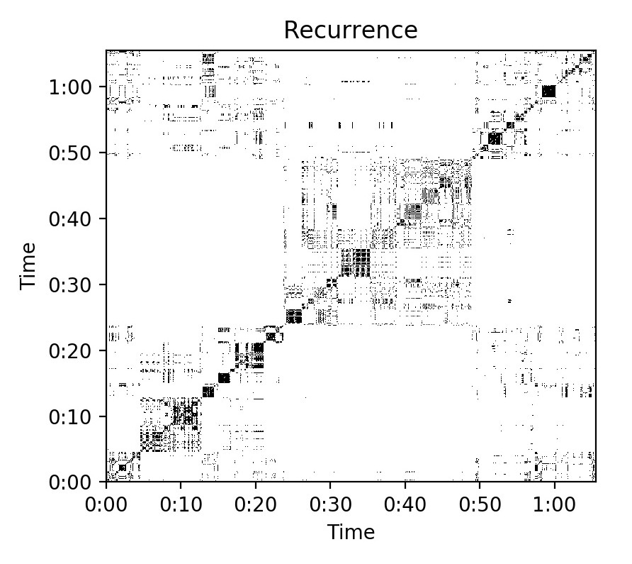
IMAGE 4.4.1: Recurrence matrix visualisation for libLLVMAMDGPUDesc.a.wav.

I followed this line of inquiry and made a thread on the FluCoMa discourse asking how I might approach segmentation based on these types of visual representations, and if any existing tools were based on a similar principle. The thread is titled “Difficult segmentation”. Owen Green responded (see IMAGE 4.4.2), elucidating that the fluid.bufnoveltyslice~object was based on Andrew Foote’s novelty-slicing algorithm (Foote, 2000), which at its core uses the notion of self-similarity represented through recurrence matrices to perform segmentation. It facilitates this by first calculating the recurrence matrix by comparing analysis windows to each other recursively. The recurrence matrix aims to describe the differences between each point in time to every other point in time. The algorithm then slides a window (the kernel) over this data, calculating from one moment to the next the summation of the differences. Together, these summaries form a one-dimensional time series, a novelty curve. From this, one can estimate times of significant comparative distance, by looking for peaks. An example of a novelty curve can be found in IMAGE 4.4.3, extracted from Foote (2000, p. 454).

A powerful aspect of novelty slicing is that the sliding window can be expanded or contracted in order to measure change across larger or smaller scales of time, respectively. Furthermore, the algorithm is relatively indifferent to the nature of the data, and thus to what might indicate novelty or salience. This makes it a popular technique for analysing the structure of music, based on the notion that points of change are not necessarily demarcated only by localised features, but also by those which are accrued over meso- and macro-scales. Given these qualities, novelty slicing seemed like the ideal algorithm for slicing my samples containing complex, but nonetheless clearly structured, musical ideas.

IMAGE 4.4.2: Owen Green answering my question in the FluCoMa discourse.

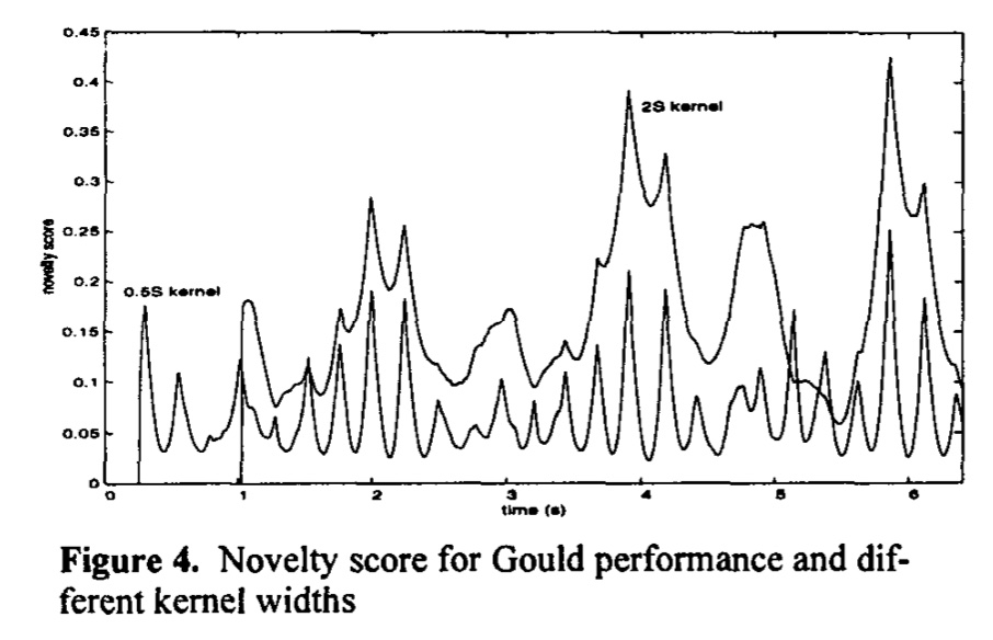
IMAGE 4.4.3: Example of a novelty curve, taken from Foote (2000, p. 454).

Using a threshold of 0.61, kernelsize of 3, filtersize of 1, fftsettings of 1024 512 1024, and a minslicelength of 2, I produced the segmentation which can be seen in AUDIO 4.4.5. To me, this segmentation result was commensurate with my initial intuitive approach seen in AUDIO 4.4.4. While at some points the results of fluid.bufnoveltyslice~ were over-segmented (slices one to five), it seemed that the algorithm could discern the changes I perceived as salient, and was able to extract the longer musical phrases such as slices seven and twelve without suffering from the oversensitivity issues found in other algorithms.

I then segmented every item in my corpus with these settings, accepting that some files might be segmented poorly because I did not want to spend an indefinite amount of time working only on segmentation. This produced 21,551 samples in total after the sounds had been processed.

Analysis

The next stage involved analysing the segmented samples. I planned to use audio descriptors that I was comfortable with and had used before, such as spectral centroid, loudness, pitch, and spectral flatness. However, I also wanted to focus on the textural qualities of the corpus items and to capture their morphological properties through analysis. This led me to use MFCCs because they are robust against differences in loudness and are capable of differentiating the spectral characteristics of sounds. For each corpus item, an MFCC analysis was performed using fluid.bufmfcc~ with an fftsize of 2048 1024 2048, numbands of 40, and numcoeffs 13. I then calculated seven statistics: mean, standard deviation, skewness, kurtosis, minimum, median, and the maximum, and up to the third derivative for each coefficient. I anticipated that calculating the derivatives of the statistics would capture the morphology of the sound by describing both the change between analysis windows as well as the change in that change. These statistical summaries were flattened to a single dimension and each column of these vectors, containing 273, values were standardised.

The analysis script can be found here: /Projects/Reconstruction Error/Supporting Code/python_scripts/descriptor_analysis/6_mfcc.py.

Dimension Reduction

In other sound-searching and corpus-exploration research, dimension reduction has been employed to transform complex data such as MFCCs into simpler and more compressed representations. Examples include the work of Stefano Fasciani (Fasciani, 2016a; Fasciani, 2016b), Flow Synthesizer (Esling et al., 2019), AudioStellar (Garber et al., 2020), Thomas Grill (Grill & Flexer, 2012), LjudMap (Vegeborn, 2020), and the previously mentioned FluidCorpusMap.

Using this research as a basis for my own work, I used the Uniform Manifold Approximation and Projection (UMAP) algorithm and reduced the 273 points in each vector for each sample to 2 points. This way, I could visualise the results as a two-dimensional map where each sample would be represented as a singular point. A strength of UMAP is its potency for capturing non-linear features in data compared to algorithms such as Principal Component Analysis (PCA). Due to the noise-based and complex spectral profile of the sounds I generated from databending, being able to capture the non-linear features of their MFCC analysis was an important consideration. Furthermore, UMAP can be coerced to favour either the local or global structure of the untransformed data by altering the minimum distance and number of neighbours parameters. A number of projections that were made with various parameters can be seen in DEMO 4.4.1. One can interact with this demo by moving the slider to interpolate between projections where different parameters for the UMAP algorithm have been used. Each point in this space represents a sample, and the interpolation is calculated based on the position of the same sample in each projection, rather than by shifting the projection based on the nearest points. This shows how changing the parameters can drastically alter the representation and grouping of sounds. I found that this was an expressive interface for changing how the computer represented the corpus analysis data.

The topology of the projections became a source of compositional inspiration involving my observation of the location, shape and relationships between clusters of samples. Some projections favoured spread-out and even distributions, while others emphasised curved and warped topologies, with samples tightly articulating these features. As well as observing these outputs visually, I explored them using a Max patch to move through the space graphically, playing back samples that were closest to the mouse pointer. Most importantly, I found that the projections performed well in positioning perceptually similar samples close to each other in the space.

This success was dependent on the parameters of the UMAP algorithm, and I experimented with several different combinations. I found that configurations with small minimum distances and a relatively high number of neighbours created projections where individual samples in close proximity to each other were perceptually similar, but nearby clusters were not necessarily as coherent. In other words, I encouraged UMAP to preserve the local topology at the expense of warping the global topology. I chose this approach because I was not interested in how all of the samples were related; rather, I wished to determine which perceptually relevant groups existed within this large corpus. That said, the projections still functioned effectively as a way of rapidly overseeing the corpus, and discerning its nature from the mass of spatially organised points. Up to this point, I had not listened deeply to the sounds in the corpus and was operating in good faith that there was indeed a collection of rich sounds in the corpus.

In this way, the computer biased my first engagement with the corpus as a unified collection. In particular, the spatial characteristics of the UMAP projection encouraged me to navigate and listen to sounds within their respective topological clusters. What I discovered through this was that there was a wide variety of variation across the corpus, and in particular, those clusters distributed far away from the central mass occasionally would contain extreme outliers, such as ner.dat.wav. These samples tended to have simplistic and static morphologies, and were less spectrally complex compared to the rest of the corpus. In a sense, they sounded like they were produced by a “broken” computer, if we are to assume the rest of the corpus was derived from a working machine. I was inspired by this initial form of soundful exploration to explore the notion of clusters further.

Future processes were all calculated on a single projection with a minimum distance of 0.1 and 7 neighbours. The dimension reduction script can be found here: /Projects/Reconstruction Error/Supporting Code/python_scripts/dimensionality_reduction/_dimensionality_reduction.py.

Clustering

Part of my affection for dimension reduction outputs was due to how samples with similar perceptual qualities were drawn together. I wanted to explore this notion computationally, and have the computer create groups of samples without my having to explore the space through manual audition. I imagined this type of output would be useful as a starting point for composing with small collections of material that the computer rendered as meaningful groups.

To do this, I first trialled several clustering algorithms on the dimension reduction output, including k-means, HDBSCAN and Agglomerative Clustering. Each algorithm exposes a different interface for influencing the clustering process, and will cluster input data based on its own set of assumptions. K-means, for example, operates by partitioning data into a fixed number of divisions set by the user. Individual points are then drawn into these partitions to create clusters. The assignment of points towards the partitions assumes that the data is spherically distributed, and that each partition will contain approximately the same number of items. This can be a problematic assumption, and a number of false conclusions can be drawn if these limitations are not accepted and acknowledged beforehand. HDBSCAN, on the other hand, determines an appropriate number of clusters automatically, depending on a set of constraints that calculate the linkage between data points. It uses a minimum spanning tree to divide the space hierarchically into clusters and so it can often respect the presence of nested structures within a larger dataset, while k-means will largely ignore such nuances. HDBSCAN can also be more suited to data that is not spherically distributed.

The differences in interface and underlying implementation between such algorithms afford contrasting insights and outcomes from this process. I found the notion of asking for a specific number of clusters from k-means potentially valuable, because I could determine approximately the density of each cluster, and thus how much compositional material a single group would contain. For example, if I wanted to create more specific groupings, I could simply ask for more clusters. However, HDBSCAN’s minimum spanning tree data structure intrigued me as an output that might guide my navigation between samples in the corpus. Inspired by the depictions of these data structures, I imagined “hopping” between connected samples in the tree, potentially using this as a way of structuring material in time. An example of a minimum spanning tree can be found in IMAGE 4.4.4. Furthermore, minimum spanning trees are not necessarily flat, and can convey a sense of hierarchy between clusters as they contain fewer samples. This hierarchical property of the minimum spanning tree is portrayed in IMAGE 4.4.5.

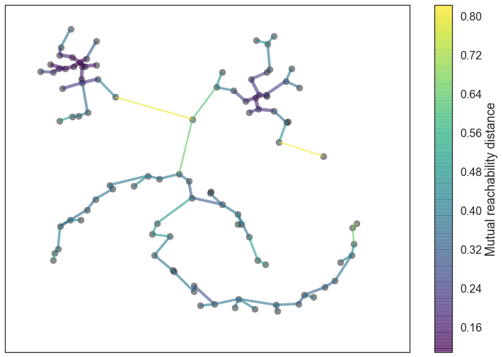
IMAGE 4.4.4: HDBSCAN minimum spanning tree visualisation. Data points are represented by circular nodes in the space with connections of the tree indicated by lines connecting them. Taken from https://hdbscan.readthedocs.io/en/latest/how_hdbscan_works.html.

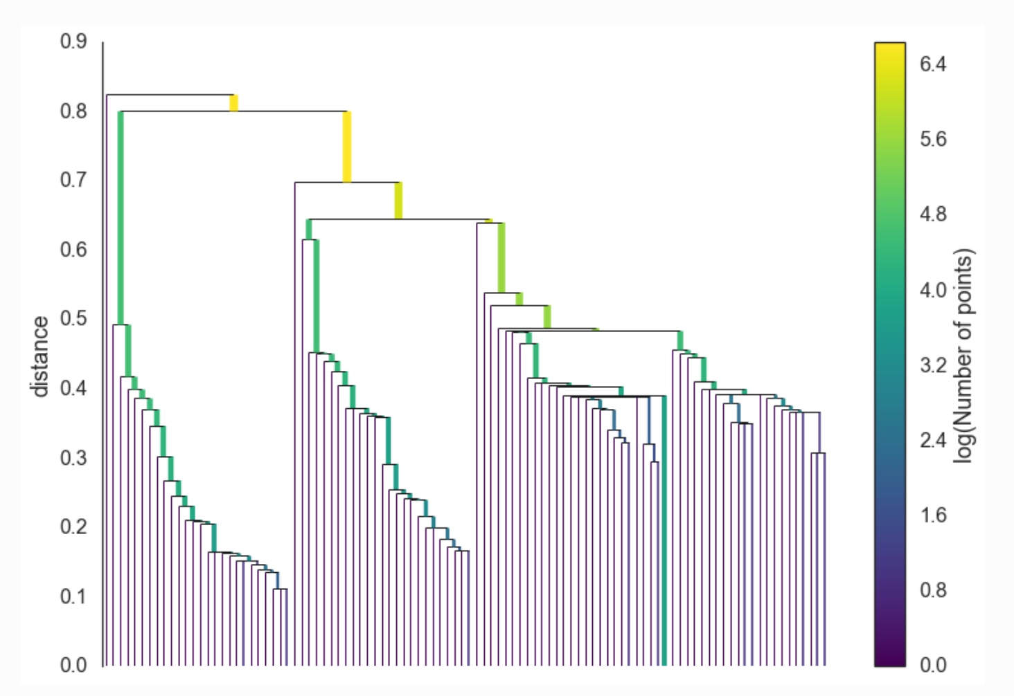
IMAGE 4.4.5: HDBSCAN cluster hierarchy visualisation. Taken from https://hdbscan.readthedocs.io/en/latest/how_hdbscan_works.html.

I settled on using another algorithm, agglomerative clustering, which can be configured to produce a fixed number of clusters, while also working in the same fashion as HDBSCAN and creating a minimum spanning tree. It is also a hierarchical clustering algorithm, making it effective when operating on non-spherically distributed and nested data, such as that produced by the UMAP algorithm. This blend of the other algorithms would allow me to control the specificity of the clustering process, while also having the computer make fewer assumptions about the distribution of my data.

Despite the initial appeal to me of the minimum spanning tree, I found it difficult to probe at the data structure which represented it in the scikit-learn implementation. I imagined that there would be a simple way to traverse the hierarchy of nodes, such as those represented in IMAGE 4.4.5 However, the methods which are exposed in the class definition for the Python module that contain the functionality for agglomerative clustering are more abstract than that, and require building one’s own traversal scheme. Although I had used Python in Stitch/Strata, I still lacked certain fundamental knowledge specific to Python as well as experience in algorithms and data structures.

Nonetheless, I was influenced by this model of relating different clusters to each other via a hierarchy. I explored this in my own way, using the agglomerative clustering algorithm to calculate four results on each projection with increasing levels of cluster density. The first output produced 250 clusters, then 500, then 1,600 and finally 3,200. These were chosen in relation to the total number of corpus items. DEMO 4.4.2 uses a small synthetic dataset to demonstrate how this clustering approach operates. The colour of each point in the visual space represents its membership of a cluster. By toggling between the three different levels of granularity (2, 4, and 8 clusters), one can observe how certain points remain together or are separated into new groups.

I then performed a series of “meta-analyses” to discern how the membership of samples to clusters changed across each level of analysis. The aim of this was to observe how modifying the number of requested clusters in the algorithm would affect the samples to the clustering process, and if I could generate my own hierarchical structure from this.

I reasoned that as more clusters were asked for across analyses, clusters at the least granular level (250 clusters) would progressively bifurcate, and samples would be separated into more specific groups. For example, the 250-clusters analysis might produce a cluster containing five samples. In the 500-clusters results, these same five samples might not belong to the same cluster. Instead, they might be spread across two unique clusters.

To evaluate this, I created a Python script that iterated through each cluster in each level of analysis in order of granularity (250, 500, 1600, 3200). As it did this, it evaluated how many samples from a cluster at one level were present in any of the clusters at the next level of specificity. The output of this meta-analysis process was three JSON files. In CODE 4.4.1, a portion of the analysis describing the shared membership of the 250-clusters and 500-clusters analysis is shown. The information in this example shows that cluster 36 in the 250 clusters analysis shares eight samples from cluster 317 and 16 samples from cluster 327 in the 500-clusters analysis. Be aware that the cluster value itself is arbitrary. The full analysis is located at /Projects/Reconstruction Error/python_scripts/clustering/cl_one.json.

{
    "36": {
        "317": 8,
        "327": 16
    },
    "89": {
        "277": 52,
        "105": 82,
        "491": 34
    },
    "70": {
        "39": 63,
        "214": 75,
        "425": 15
    },
}

CODE 4.4.2, shows a portion of the meta-analysis of shared cluster membership between the 500-clusters and 1600-clusters outputs. From this one can discern that cluster 313 from the 500-clusters analysis shares 22 samples with cluster 1,256 in the 1600-clusters analysis.

    "313": {
        "1256": 22
    },
    "327": {
        "19": 10,
        "994": 6
    }

Using both of these analyses together, one can discern that there is a relationship between clusters 36, 327 and 19 from the 250-clusters, 500-clusters and 1600-clusters analysis respectively. They all share, to some extent, similar materials and one might consider cluster 19 to be a sub-cluster of 327, which itself is a sub-cluster of 36. In fact, I found later in the compositional process that this way of relating the clusters was perceptually meaningful. By accessing the levels of this sub-cluster hierarchy, I could discover varying degrees of perceptual similarity and tightness. I could start with a broad top-level sample in the 250-clusters analysis, and follow the linkage in the meta-analysis to derive sub-clusters with more perceptually defined groups of sonic materials. This became essential to how I first engaged in audition with these sounds, and how I composed and structured several of the pieces.

The clustering code can be found here: /Projects/Reconstruction Error/Supporting Code/python_scripts/clustering/_clustering.py and the meta-analysis script can be found here: /Projects/Reconstruction Error/Supporting Code/python_scripts/clustering/hierarchical_cluster.py.

Moving Forward

At this stage, I moved into soundful play with the various computer outputs which led the development of the pieces. The next section [4.4.3 Responding to Computer Outputs] discusses this.

Responding to Computer Outputs

After producing the clustering data and the meta-analysis, I used it to drive audition processes in Max and REAPER. I created an interface that allowed me to retrieve the samples from a specific cluster, and simultaneously navigate between clusters that shared samples, determined by the meta-analysis. This facilitated a listening process in which I would start with a cluster of samples from the 250-clusters analysis, and curate the samples by selecting sub-clusters of that initial cluster. The samples were played back contiguously by a sequencer, so that I could rapidly ascertain an idea about the perceptual qualities of each cluster. Through this approach, the computer led me to perceptually constrained groups of sounds. A screen capture demonstrating this auditioning process can be found in VIDEO 4.4.10.

This process was immensely useful for becoming acquainted with the corpus samples in a structured manner. Even though the source material was generated from disparate sources of raw data, this structured engagement mediated by the computer’s analysis began to catalyse higher-level compositional thinking for what an EP of different pieces might present. As I was auditioning with this Max patch, I created a set of annotations for each cluster and my own set of “tags” describing the perceptual qualities and imagined compositional applications. These tags range from noting which samples I thought were similar, to devising forms based on the relationships between the groups. These notes can be found at this link: cluster notes.

Up to this point, the audition process was orchestrated entirely in Max. However, I did not want to compose in this environment because I was beginning to formulate concepts around formal structures and the way these samples would be constructed into a set of compositions. Working entirely in Max had already proven to be problematic in Stitch/Strata, especially in the earlier phases of that project. Instead, I wanted to be able to access samples as clusters in an environment where I could “freeze” them, arrange them, as well as modify and alter them with audio effects. To achieve this workflow, I built a series of Lua scripts that allowed me to turn a cluster represented in JSON format into a track in REAPER by leveraging the ReaScript API. This can be found in CODE 4.4.3.

local info = debug.getinfo(1,'S');
local script_path = info.source:match[[^@?(.*[/])[^/]-$]]
package.path = package.path .. ';' .. script_path .. '?.lua'
package.path = package.path .. ';' .. script_path .. 'lunajson/src/?.lua'
loadfile(script_path .. "../ReaCoMa/lib/reacoma.lua")()
local lunajson = require 'lunajson'

local confirm, user_input = reaper.GetUserInputs(
    'Provide JSON info', 
    2, 
    'JSON Path:, Cluster Number:, extrawidth=100', ''
)

if confirm then
    reaper.Undo_BeginBlock()

    -------- start processing --------
    reaper.SetEditCurPos(0.0, false, false)
    reaper.InsertTrackAtIndex(0, true)

    -- Parse user input --
    local fields = reacoma.utils.commasplit(user_input)
    local json_path = fields[1]
    local cluster_num = fields[2]

    -- Do JSON parsing --
    local file_in = assert(io.open(json_path, "r"))
    local content = file_in:read("*all")
    local cluster_data = lunajson.decode(content)
    for k, p in ipairs(cluster_data[cluster_num]) do
        reaper.InsertMedia(
            '/Users/james/Cloud/Projects/DataBending/DataAudioUnique/'..p, 
            0
        )
    end
    reaper.SetEditCurPos(0.0, false, false)
    reaper.Undo_EndBlock("Insert Media Cluster", 0)
end

Running this script would present me with the option to provide a JSON file and a cluster number. This would generate a new track containing the samples belonging to that cluster. This allowed me to audition samples rapidly in Max, then draw them into a REAPER session without friction. VIDEO 4.4.11 demonstrates this process. This was the basis on which I composed the next few pieces. I would oscillate between listening in Max, importing sounds into REAPER as clusters, and then using intuitive compositional processes to organise that material. When I hit a creative block in the DAW, I would return to listening and try to find something new in the material, guided by the computer.

The next sections, [4.4.3.1 _.dotmaxwave], [4.4.3.2 —isn], [4.4.3.3 X86Desc.a], [4.4.3.4 segmnoittet], and [4.4.3.5 sys.ji_], describe the specific compositional processes for each piece in Reconstruction Error and how the computer informed my compositional choices and led the compositional process.

_.dotmaxwave

_.dotmaxwave was the first piece I composed. The samples that I used to create it were all derived from cluster 131 from the 250-clusters analysis. While auditioning this cluster in Max, I realised that the source material was all derived from a particular raw data type with the .maxwave extension and possessed similar morphological properties. All of the samples begin similarly, with four repeated pitched sounds leading into a static texture. These can be heard in AUDIO 4.4.7. This static texture contains a predominant pitch component with some quiet and narrow-band noise. I wanted to capitalise on what I had found to create a track that focused on the relationship between pitch and noise, as well as the shared morphology of these samples.

I started by importing cluster 131 into REAPER. I listened to the samples and identified those that I found to have the most novel variations in the opening sequence. From this, I was able to create a palette of iterations on the same musical idea.

Using the Fluid Decomposition Toolbox harmonic-percussive source separator, fluid.bufhpss~, on the command line, I processed each of the sounds. I achieved a clear separation of these two elements using this technique and found that the percussive components had their own complex morphology and character. However, in the unprocessed version of the samples this component is low in volume and masked by the more dominant pitch sound. I wanted to emphasise the noise component, so I summed the two components back together after increasing the volume of the noise.

The rest of the piece grew from this concept and workflow. I would decompose different samples with the harmonic-percussive source separator, and then listen to these outputs in isolation. This process guided how I structured the piece and how I selected different samples intuitively. The first section, from 0:00 to 1:13, highlights the morphological characters of a number of variants, while the remainder of the piece draws on the decomposition process to structure different presentations of percussive material buried within these samples. The final crescendo, from 2:25 to 3:37, uses a sample that had the most intricate and dynamic material noise component, which before the decomposition procedure was concealed by its harmonic component.

While composing this first piece I had to work constantly outside REAPER to perform decomposition processes. It was tedious to have to leave the DAW to perform audio processing as well as constantly structuring command-line invocations, navigating the file system and the DAW timeline in order to set up the necessary media items for audition and composition. This friction led me to create ReaCoMa, a set of ReaScripts that bridge the Fluid Decomposition Toolbox command-line tools to REAPER. These scripts allow one to process media items directly in REAPER, and to configure the parameters of various decomposition algorithms such as harmonic-percussive source separation, non-negative matrix factorisation, transient extraction, and sinusoidal isolation with a graphical user interface. In addition to this, the segmentation algorithms from the toolbox are bridged, allowing media items to be partitioned using several different approaches to dividing sounds in time. In the remaining pieces of Reconstruction Error, ReaCoMa played a vital role in unpicking the internal content of sounds, once I had discovered and selected them through analysis. It also led me to perform additional segmentation to restructure sounds in time.

—isn

—isn is composed using clusters of samples with short impulse-based material. While composing I was often using the notes I made for each cluster as a way of informing me of what samples to experiment with next. I noticed that I classified a large number of clusters as “short”, “fast” and “delicate”. This specific portion of my cluster notes can be read here: /Projects/Reconstruction Error/Supporting Code/clusters.md.

I selected these specific clusters and auditioned them by playing samples back-to-back in a sequencer-like fashion. The repetition of impulses formed rhythmic patterns, where the length of the samples and their inherent differences in morphology contributed to subtle and unique musical objects. From this method of arranging samples, the internal dynamics of each cluster were foregrounded and I wanted to capitalise on the tension this created between the tight perceptual grouping of each cluster, the slight differences between the samples within a cluster, and the overall perceptual separability between clusters.

Thus, the piece is structured around the superimposition of several of these loops, which are individually derived by concatenating samples from distinct clusters. This approach was in part influenced by Robert Wannamaker’s piece I want to tell you something… (1999), which uses the summation of several sinusoidal components to build a noise texture. The structure of this work is built on realising this process slowly over time, and allowing the listener to be engaged with moment-to-moment repercussions of combining highly constrained, atomic units of sound. This approach resonated with my relationship to the impulse-based material.

From 0:00 to 2:34, I created a passage of gradually increasing intensity and textural complexity by taking several of the clusters and applying linear fades. Some clusters are more similar than others and layering them in this way creates subtle phasing and otoacoustic effects, reminiscent of those one might find in Thomas Ankerschmidt’s compositions or Olivier Pasquet’s work with impulse-based material. As more layers are introduced and their unique dynamic and textural properties interact with each other, different layers become harder to unpick from one another, and the musical surface becomes denser and more complex. The relatively abrupt break at 2:34 reduces to just two of these layers, significantly decluttering the texture and constructing a much sparser musical behaviour. The remainder of the piece explores this stripped-back and reduced sound world, only ever superimposing two or three clusters at any one time.

I imagined that I might proliferate the musical ideas I had built up to this point. However, I could not derive any more novel superimpositions of clusters that I found satisfactory and envisaged that to continue the piece I would need to introduce more material or to move in another musical direction. I decided to keep the material constrained only to the clusters I had initially grouped in my annotations and thus to keep the piece tightly focused on my initial idea.

X86Desc.a

X86Desc.a iterated on the material types used in —isn. It focuses on the incorporation and treatment of similar sound types but expands the palette of transient-based material through processing spectrally complex sounds from other clusters in the corpus with ReaCoMa.

For example, the material at 0:45 is created using a transient-extraction algorithm from ReaCoMa. The source material, libLLVM-6.0.dylib_144.wav, is predominantly pitched and the result is perhaps not recognisable as derived from the source material due to the removal of the non-transient component of that sound. This process is used throughout the piece to generate different materials. Depending on the morphological properties of the input sound, a number of different quasi-rhythmic patterns are carved away from the spectrally rich sources. For example, at 2:07, one layer of the overall texture was derived by taking a cluster of samples and processing them through the transient-extraction algorithm. I did this with three different settings, to create variations on that material, which I then used to formulate a morphing passage of sound. This is presented in AUDIO 4.4.10.

In isolation, the results of these types of decomposition processes were uninspiring to me, and the musical effect was underwhelming. However, I found that by layering multiple instances I could create complex interactions between different streams of transient-based material. The rest of the piece was intuitively composed around my experimentation with this decomposition and layering process. Overall, this piece contained all of the trailing ideas that I did not want conceptually to pollute —isn with. For me, the results were sufficiently distinct to warrant my making a new piece in the album, although the mechanics of composing the piece were quite similar.

segmnoittet

For this piece, I wanted to create something that was less rhythmically homogenous than the previous tracks and to create something more mechanical and sparse. The first idea I had involved taking clusters that, when concatenated, would create such aspects inherently and without much low-level editing. I found that sample groups often created such results through sequencing if the samples within a cluster had significantly differing lengths. I was able to control and search for this aspect by selecting samples from different hierarchical levels of the meta-analysis. The deeper I went into the hierarchy, the more similar samples were in both duration and perceptual quality. As such, “high-level” clusters would be more variegated and mixed, while “low-level” clusters were highly constrained and repetitive. A short section of music composed in response to this finding can be heard in AUDIO 4.4.12.

This passage did not develop successfully and I had exhausted a lot of the material which I had collected up to this point. Most, if not all, of this material was derived from cluster 250, so I started following the connections that this cluster had to the other outputs via the meta-analysis. This did not introduce many additional samples, though it did separate the same or similar material into more specific clusters. In IMAGE 4.4.6, the REAPER session of this piece is shown, indicating tracks where each child cluster is positioned alongside its parent cluster into the session. These are colour-coded to represent the shared membership and are annotated such that I could discern from which output they originated.

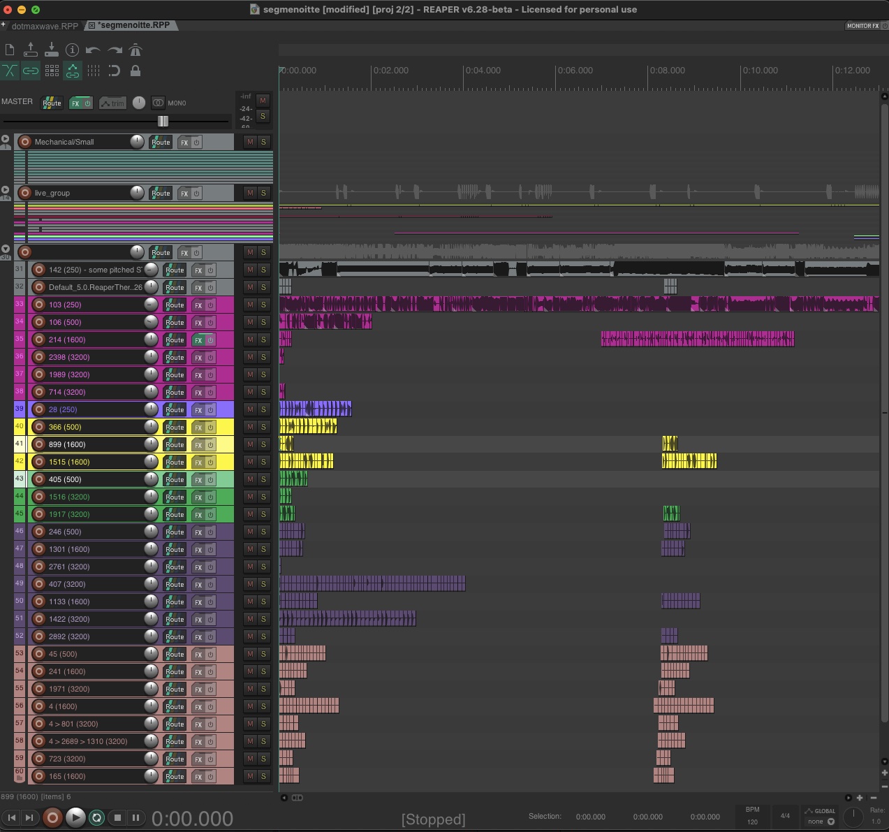
IMAGE 4.4.6: REAPER session for segmnoittet. Tracks displayed on the left side of the screen contain various tracks of clusters and their respective "sub-clusters".

After importing these clusters, I was able to keep composing, and eventually the compositional process took a new direction. The overall aesthetic became much more relaxed and less rhythmically assertive and block-like. The presentation of short gestures became much more reserved than before, as many of them were superimposed or more sparingly used to ornament longer textural sounds. I was able to create various effects by carefully selecting perceptually homogenous groups of materials and treating them as individual compositional units. I used the hierarchy of clusters to control how constrained each of these compositional units were. For example, at 1:10 a small cluster is processed with a filter. The original impulses in this small section of source material are bright and contain lots of high-frequency content, so the result is “punchy” and sounds almost overdriven. This individual gesture results from the concatenation of a novel sub-cluster which I encountered after importing the clusters into REAPER from the 3,200 clusters group. The static texture at the start is created by taking similarly constrained samples that were short in duration. Thus, their concatenation creates a pitched and stable quality. At various time points (0:25, 0:35 and 0:40, for example), small gestures function as interjections to this static texture. Each of these interjections is derived from clusters in the 500-clusters output and they are relatively varied in comparison to the static texture upon which they are superimposed.

The slowly unfolding ending is created by taking another sub-cluster, and arranging the samples in the REAPER timeline so that the interval between samples gradually expands. This process is duplicated several times and superimposed.

At the beginning of this process, the spacing between individual samples is small, and their repetitious arrangement generates material that has a strong pitched element. This spacing expands over time, which produces a sonic effect in which this pitched element disappears, and consecutive samples become impulse-like. To orchestrate this, I created a Lua script that could interactively distribute items in the REAPER timeline. This script allowed me to set a fixed spacing between media items, as well as a noise factor that could skew those items along that temporal structure. This is demonstrated in VIDEO 4.4.12, in which I take several impulse samples and modify the spacing between them.

sys.ji_

This was the last piece that was composed for the album. It is the most distinct in terms of compositional approach and material used. For me, it signified a developmental milestone in the compositional process, where I was comfortable enough with the corpus that I could navigate almost intuitively and directly towards certain material types. Instead of entirely relying on the computer to seek out sounds, or to be offered potential groupings, I used the knowledge I had accrued by composing the other four pieces. Three of the other pieces, —isn, segmnoittet and X86Desc.a, are composed almost entirely with short impulse-based material. The way I structured these sounds focused on their delicacy and fragility, as well as on their quasi-rhythmic and interlocking nature through concatenation. I wanted to compose an antagonist to these pieces, and to draw on materials from the corpus with bombastic and spectrally rich qualities.

When I was experimenting with different clustering algorithms, I trialled another algorithm, HDBSCAN, which is discussed in some detail in [4.4.2.5 Clustering]. One cannot direct HDBSCAN to produce a specific number of clusters; rather, it determines this for itself in response to a number of constraints built into the algorithm. I found this clustering technique much worse in terms of perceptual similarity, and the clusters often contained only two or three samples even when adjusting the parameters drastically. While the results of the clusters were unsatisfactory, HDBSCAN is novel in that it produces a cluster containing samples it cannot confidently assign membership to. In theory, this cluster should contain samples that are statistical outliers, which in terms of perception, would suggest that they may be unique or novel compared to the rest of the corpus. I auditioned this outlier cluster and found noise-based, chaotic and spectrally complex sounds. While this morphological and textural quality was abundant in other samples in the corpus, the samples in this particular cluster expressed their own particular variant of it. Noise in these samples was often densely layered, like a carefully constructed field recording of machine-like source material. This contrasted to the often unrelenting, harsh and broadband noise that was present in many other corpus items. I noticed that several of the samples in this outlier cluster had originated as segments from the file sys.ji_.wav. I isolated a group of these that I instinctively liked, and worked backwards by examining the agglomerative clustering data to see where those files had been grouped by that algorithm. This led me towards other noise-based samples that were not present in the HDBSCAN outlier cluster. In effect, I used the two different clustering algorithms as a mechanism for discovery through cross-referencing.

This hybrid approach revealed to me how the curation of algorithms and technical implementation can be instrumental as an expressive tool. Each of the clustering algorithms produced different representations of the corpus, and through their differences I was afforded a novel method of corpus exploration, leading to the incorporation of new samples into the piece. The first half of the piece uses segments from sys.ji_.wav, and as material develops around 1:18, samples derived through cross-referencing are gradually included. These samples are more striated and iterative, and start to display shades of subtly filtered noise, as well as some pitched components. This high-level structural change is emphasised at 2:34, in which a totally new category of noise samples are presented that are derived from source files with the .reapeaks extension.

Reflection

Reconstruction Error was a major point of development in this PhD, in terms of compositional workflow and the relationship that developed between me and the computer. The balance of agency was more equal than it has been in other projects – at times, I composed entirely intuitively, and sometimes I was responding reactively to the outputs of the computer – allowing technology to lead my decision-making. This fusion of my musical thinking and the computer’s numerical and machine listening was one of the most successful aspects of this project.

Clustering was significant in this respect and structured my engagement with the materials of the corpus hierarchically. As a result, the forms of the works emerged as responses to the structures encoded into the clustering hierarchies, and from what I was able to discern from the comparison of several different outputs. This aligned conceptually with my wider approach to form, as described in [2.2.3.1 Form and Hierarchy].

Furthermore, decomposition processes afforded by ReaCoMa were essential to the way that I derived novel sounds as well as conceiving of concepts and formal structures. This is preeminent in _.dotmaxwave, which is structured in response to my decomposition of sounds with the maxwave extension. X86Desc.a also emerged as a response to the results of transient extraction.

By engaging in these forms of dialogue with the computer, the creative process was undertaken mutually and the computer inflected my compositional decision-making. This allowed me to hone my creative thinking and to transform my surface-level appreciation for the databending practice into a project in which those ideas are incorporated authentically and in a personalised manner.

Being able flexibly to put aside, or to work entirely with the computer, encouraged me to compose more radical and daring presentations of material. In the previous projects in this PhD, my focus had been more formalistic, trying to make the computer structure the formal organisation of material through constraints or algorithms that modelled compositional decision-making. This was restrictive because each and every idea was mediated through the lens of how it could be encoded into a programmatic representation. I was not constrained by this in Reconstruction Error, and the computer played the role of leading me or taking on the role of a compositional provocateur. As a result, each piece feels to me more conceptually focused, because I could devote the necessary creative resources to pursuing specific ideas, rather than merely engaging with them as a byproduct of technical work or their being fully realised only after the fact.

Shifts in Technology

A key development in my practice that emerged in Reconstruction Error is the shift towards using Python and the DAW as a combined compositional workspace. This combination had been used in Stitch/Strata and I reflected on the positive aspects of this technology in [4.1.3.1 State and the Digital Audio Workstation].

Returning to this combination in Reconstruction Error proved effective because it balanced the interactive aspects in a way where I could step between the mindset of listening, soundful experimentation and compositional decision-making without those things necessarily being intertwined temporally.

As an analogy to flesh out this idea, my workflow could be contrasted to that of the live coder, who inputs their commands to the computer in real-time and listens to the response in order to guide their future actions. Such reactions and interactions are determinant of what will happen next musically. The workflow in this project separated immediate soundful musical action and play from the compositional and conceptual thinking mediated by the computer.

When I was engaged with musical materials in the DAW I could stretch, compress, shift, cut and reorganise the temporal aspects of the pieces separately from the other elements of my workflow. Thus, the building blocks of that process are selected and navigated out of time through structured listening by the computer. On reflection, I realised that this is an essential aspect of how I want to interact with the computer to make music.

Finding Things In Stuff

The success I found using Python and REAPER motivated me to create a software framework for facilitating and developing this workflow for future projects. Much of the code I had written for this project would have been difficult to use for other projects. Elements such as hard-coded paths, a non-standardised file structure for keeping corpus materials, and a general inflexibility in the code meant that it would be much easier to start afresh. Similarly, a majority of the iterative back and forth was not captured in the artefacts which remained at the end of the project. Towards the end of Reconstruction Error, scripts were made to use configuration files instead of command-line arguments, and these act as a form of automatic recording keeping for what I did in the creative process. Generally, it remains difficult to retrace the steps of the compositional process and to understand how things changed over time. This is largely a consequence of not knowing in the moment if something I am doing is going to be significant later. Ideally, these aspects are abstracted away so that a consistent record is maintained at all times by the computer.

In response to this need, I began to develop FTIS, an extensible Python-based computer-aided composition framework for machine listening and machine learning fostering integration with REAPER and Max. Instead of relying on “single-use” scripts, FTIS was designed to facilitate the construction of computer-aided processes as extensible and flexible pipelines of connected components that are useful in the creative process. I outline the capabilities and possibilities of FTIS in the relevant section in [5. Technical Implementation and Software], as well as explaining the underlying architectural aspects that serve my compositional thinking and workflow.

Final Remarks

The next project, Interferences, is the final project in this PhD portfolio. It incorporates FTIS extensively and indeed informed the development of early versions of that software.

Musically, Interferences draws on a similar digital and synthetic sound world to Reconstruction Error. It also continues to explore how the computer can be engaged in a creative dialogue by leveraging dimension reduction and clustering. This is explored in much more detail compared to Reconstruction Error, facilitated by the flexibility of FTIS. That said, the treatment of compositional material is different to that in Reconstruction Error, and I focused in the later project on creating longer-form works.

Further Information

I gave two presentations that discussed Reconstruction Error at different points in its development. The first presentation was at the November 2019 FluCoMa Plenary, where the pieces were partially composed, and I focused on demonstrating my application of the FluCoMa tools. This can be seen in VIDEO 4.4.13. Much later, after the pieces had been finished and after I had moved on to composing Interferences, I reflected on the entire development process of Reconstruction Error and its relationship to the compositions themselves in a short paper and presentation for the 2020 AI Music Creativity Conference. This involved creating a short video demo, which can be viewed in VIDEO 4.4.14.