Interferences

Interferences is the fifth and final project in this portfolio. It is a pair of works presented as an EP. There is a git repository that contains all of the Python code and Max patches that were used to create the work. This repository can be found here: /Projects/Interferences/Supporting Code.

Motivations and Influences

A primary motivation for this project was to develop the workflow established in Reconstruction Error, and to build on my creative-coding practice with Python, Max, REAPER and FTIS. There were two aspects to this motivation. Firstly, I wanted to recreate the experience of navigating through a corpus of unknown materials led by the computer through structured listening. Although I only utilised a small portion of the corpus in Reconstruction Error, I wanted to generate a new corpus with its own origins, whilst still situating my work within a digital and synthetic aesthetic. At the time, I was interested in circuit bending and the vast number of sounds that breaking apart and reconstructing old electronics could generate. The aesthetic of these sounds suits my sensibilities well, and I imagined that collecting a number of them could be a path forward for creating the corpus that I needed. Tangential to this research, I came across a video of Nicolas Collins using an induction microphone to amplify the sounds of electromagnetic interferences generated by everyday appliances and objects. This video can be seen in VIDEO 4.5.1. It struck me that instead of circuit bending, this might be a suitable technique for creating a large corpus with the properties I desired. Following this hunch, I obtained an Elektrosluch Mini induction microphone capable of recording electromagnetic interference. I describe how this device was instrumental in the compositional process further in [4.5.2.1 Recording Objects with Induction].

Secondly, I wanted to iterate on the pipeline of segmentation, analysis, dimension-reduction and clustering and to apply it more fluidly to new compositional materials. The technology implemented in Reconstruction Error was successful for enabling me to be creative, but was largely inflexible and so to perform the same tasks on new material would require rewriting the scripts. Thus, FTIS was developed to support this goal, and made it possible to create scripts that supported experimentation and data manipulation. This aspect is discussed in more detail in [4.5.2.3 Pathways Through the Corpus].

Compositional Process

The compositional process for Interferences can roughly be divided into two phases. The first phase involved experimentation with FTIS and devising various ways to navigate through the corpus with the aid of the computer. The second phase involved a more direct level of composition in which I used the computer to search and hone in on specific materials in the corpus for this project. This contrasts with the broader exploration undertaken in the first phase.

Recording Objects with Induction

As outlined in [4.5.1 Motivations and Influences], I procured an electromagnetic induction microphone and wanted to use it to generate a corpus of digital and synthetic-type sounds. To do this, I took electronic objects from around the home and recorded them, at times operating those objects simultaneously. This gathering stage came before the two previously mentioned compositional phases. I was surprised by the diversity of sounds this produced. Despite devices in my environment seeming inert, the induction microphone could detect and uncover their invisible electronic signatures and traces of their operation. I recorded a number of devices, including my computer keyboard, mouse, a mobile phone, a sound card, a laptop and an e-reader. Each device produced its own characteristic outputs, and some of them offered me the ability to trigger certain sonic behaviours through my interaction. For example, AUDIO 4.5.2 captures the sound of an e-reader left relatively untouched. The change at 0:02 is triggered by switching the “aeroplane mode” on and off. This user interaction causes the components in the e-reader to operate differently, which is captured by the induction microphone. Eventually, the initial static state is returned to. This can be heard at 1:59, lasting until the end of the clip.

While other devices produced their own characteristic sonic materials, I found that across all of them I listened to, my interpretation would always coalesce around an antiphonal distinction between active and static musical states. For example, AUDIO 4.5.3 is extracted from the electromagnetic interferences of a mobile phone. In my perception of this sound, there are two sonic classes at work here, where 0:00 to 0:40 is static, and where the remainder of the recording is active.

As I recorded and browsed through these sounds, I was reminded of the work of Australian field-recording artist Jay-Dea Lopez and the way he taps into similar sources using contact microphones attached to monolithic infrastructural objects in the outback. In particular, three blog posts of his, “Low Frequencies”, “Coil pickups and microsounds” and “Raising the Inaudible to the Surface”, contain these types of material. Similarly, I felt a certain connection between my experiments and the morphologies and textures present in Bernhard Gunter’s Untitled I/92 (1993) (VIDEO 4.5.2), and Alvin Lucier’s Sferics (1981) (VIDEO 4.5.3). To me, both of these pieces shared some of the characteristics of what I was discovering with the electromagnetic microphone – delicate and fragile sound worlds full of intimate clicks, pops and spectrally constrained sonic fragments. Furthermore, these external influences started to funnel into my conceptualisation of the initial material as that which can occupy two distinct states – busy and rapidly changing or unchanging and glacial in nature. This became an essential starting point in the technological process of using machine listening to navigate through this corpus of sounds framed by the opposition of static and active states.

Static and Active Material

In the first phase of the compositional process, I began by trying to dissect the corpus into two groups based on classifying whether they were static or active. To do this, I first had to segment the corpus, and then find a way of crudely classifying those segments into either of these two categories.

Segmentation

The end goal for segmentation in this project was to divide each sound into static and active components automatically. I planned to apply a classification or clustering analysis to the segments made by this process, so that the computer could discern which categorisation each segment might belong to. This was complicated because the time span of static and active states was highly variable, to my perception, depending on the file. AUDIO 4.5.2 shows only a portion of what was created from recording an e-reader, and the static and active states last for several minutes between alternations. AUDIO 4.5.4 shows another recording taken from a wireless game controller, which demonstrates similar oscillations between static and active states, although these changes occur over seconds rather than minutes. Given these disparities in time scale, a frame-by-frame analysis was likely to be unsuitable and hard to tune appropriately to capture the sparse and specific moments in time in longer samples, while also being sensitive to the shorter-term changes.

To tackle this, I created a bespoke algorithm influenced by Lefèvre and Vincent (2011), which performs segmentation by sampling short sequences within a sound and clustering those sequences together. My algorithm, Clustered Segmentation, is structured as a two-phase process. The first phase encompasses a “preprocessing” segmentation pass, in which a sample is divided into numerous small divisions. These divisions are not necessarily perceptually meaningful; rather, the process aims to divide the signal finely into minute segments that can be recombined later in the second phase. Several different segmentation algorithms can be used at this point to perform this preprocessing. The second phase applies audio-descriptor analysis to each segment and then groups each one into a user-specified number of clusters. This number of clusters parameter determines how discerning the algorithm is in distinguishing the segments from each other. After clustering, the algorithm recursively takes a window of clustered segments and merges contiguous segments that have been assigned the same cluster label. This process starts at the first segment and shifts forward in time, merging clusters recursively as it moves along. Thus, it gradually creates ever-larger combined segments until each consecutive segment belongs to a different cluster. The size of the window of clusters (window size) in this process is also configurable. IMAGE 4.5.1 is a visual representation of this algorithm.

IMAGE 4.5.1: Visual depiction of "cluster segmentation" algorithm.

My intention here was to create a generalisable algorithm that would be relatively agnostic toward the nature of the material it was segmenting. I also wanted to avoid some of the issues whereby frame-by-frame approaches often only target short windows of time and do not respect the longer-term implications of changes in the signal. Using a shifting window that merges while it slides across the segments gives the algorithm a “lookahead” and “look behind” capacity that constantly updates as it progresses.

I evaluated the effectiveness of Clustered Segmentation by modifying each parameter of its two-phase segmentation process and observing the results as a REAPER session. Overall, my observation was that the choice of a specific segmentation algorithm for the preprocessing stage had little effect on the final result. I experimented with several flavours of segmentation from the Fluid Decomposition Toolbox (which were at this point embedded directly in Python), including fluid.onsetslice (a spectral segmentation algorithm), fluid.noveltyslice (another spectral segmentation algorithm) and fluid.ampgate (an amplitude-based segmentation algorithm). I discovered that for any of these algorithms, the most desirable outcome was one in which the source sample was segmented very finely. If the segments were too long, Clustered Segmentation would often deem contiguous segments to be similar because the data in each segment regressed to the mean. Thus, it was important that the preprocessing stage produced segments which are very short. Furthermore, the window size and number of clusters parameters had a significant effect on the results. In the development and testing phase of Clustered Segmentation, I found it difficult to predict how different combinations of these two parameters affected the result. IMAGE 4.5.2 shows the REAPER session I used to inspect the results, where each track is the result of a different parameter combination. The session itself can also be found in the repository here: /Projects/Interferences/Supporting Code/segmentation_scripts/2020-06-18 04-09-54.718681/session.rpp and the code that performed the segmentation can be found here: /Projects/Interferences/Supporting Code/segmentation_scripts/clustered_segmentation.py.

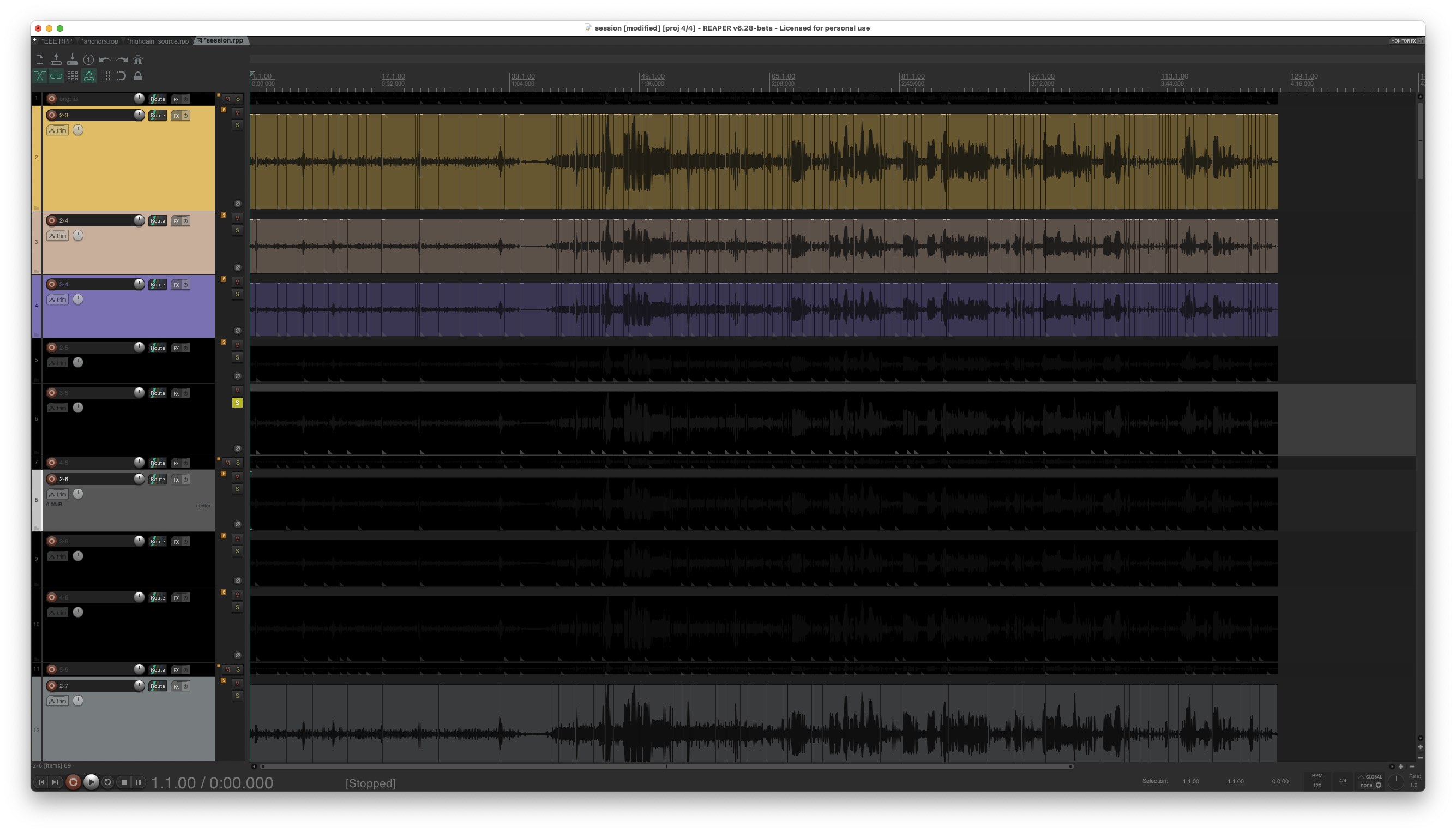
IMAGE 4.5.2: Clustered segmentation results rendered as a REAPER session.

I was hoping that the algorithm would be able to automatically detect the salient textural changes in the source materials between active and static states. Testing different parameter combinations on sounds from the corpus produced a variety of results. Some of the results were clearly unsatisfactory and there was minimal or no amalgamation of segments from the preprocessing stage. Other parameter combination results were more promising, and in many cases were harder to evaluate. In these “borderline” segmentations, points that I would intuitively discern as changes in texture and morphology had been detected by the computer. However, rarely did two configurations agree on the same set of results. Given this disparity, it was difficult to determine a “best” configuration. Moving forward, I turned this algorithm into a FTIS analyser, as previously I had been testing and developing it as a “one-off” script. I then ran the algorithm on all of the corpus items using this script: /Projects/Interferences/Supporting Code/segmentation.py. The results from this script were satisfactory but not perfect. In some cases, areas of homogeneity in the signal had been divided. However, distinct areas showing static and active traits had been detected and separated.

Classification Through Clustering

I then classified each of these newly generated segments into two distinct groups. I performed this by calculating seven statistics: mean, standard deviation, skewness, kurtosis, minimum, median, and the maximum, and their derivatives, up to the second derivative on the spectral flux across windowed frames in each corpus sound. This process was based on the same one described in [4.4.2.3 Analysis]. Using the Agglomerative Clustering algorithm (first described in [4.4.2.5 Clustering]), I then clustered each sound into one of two groups based on this statistical analysis. The code for this whole classification process can be found here: /Projects/Interferences/Supporting Code/split_by_activity.py. I examined the results by loading the clustering data into Max and auditioning sounds within each cluster separately. The results were acceptable, and I found that dynamic and texturally variegated sounds had been partitioned from those that had invariant and stable morphologies. This separation of the samples mapped on to my perceptual model of these sounds belonging to either an active or static state, respectively. A selection of different results from this process is presented in AUDIO 4.5.5.

Pathways Through the Corpus

This section describes different pathways through the corpus of segmented and classified sounds I had created, and experiments that aided in formulating concepts and ideas for the two pieces through audition and structured listening. I wanted to begin by deconstructing further those sounds classified into the active category, into individual impulses, utterances and segments. For example, I imagined that AUDIO 4.5.6, a segment from Kindle_04_08.wav, might be restructured to be less chaotic and more ordered; perhaps a rhythmic structure could be imposed upon individual segments extracted from this sound.

Following this intuitive desire, I used FTIS to segment the active sounds and then clustered the resulting segments based on their perceptual similarity. This was orchestrated with two separate FTIS scripts. Firstly, a segmentation script, /Projects/Interferences/Supporting Code/micro_segmentation.py, that uses the Clustered Segmentation algorithm to segment the active sounds. Secondly, this is followed by a clustering script, /Projects/Interferences/Supporting Code/micro_clustering.py, which calculates MFCCs for each segment and agglomerates them using the HDBSCAN algorithm. The clustering results can be found here: /Projects/Interferences/Supporting Code/outputs/micro_clustering/5_HDBSCluster.json and I will refer to them as “micro-clustering” results henceforth. I explored the results of this process in Max aurally and found that this process rendered perceptually homogenous clusters in terms of texture and morphology. VIDEO 4.5.4 captures this audition process and demonstrates the clusters’ perceptual homogeneity. This patch can be found here: /Projects/Interferences/Supporting Code/classification_explorer.maxpat.

This Max patch looped a selected sample from a cluster in the micro-clustering results. As I navigated between clusters and explored samples within them, the intricacy and fragility of the sounds within specific clusters was foregrounded. Curiously, some material that I would have perceived as static had been included in what was the active classification performed earlier. The nature of the looping playback, combined with the already mechanised and artificial quality of these sounds was evocative. I was compelled by the qualities of different groups, imagining composing with the segments to form my own artificial machine-like sound composites. Clusters 1, 2, and 37, for example, produced structured rhythmic sounds articulated by sparse and subtle transients. By changing the sample, the rhythmic patterns of these articulations could be altered. I imagined that combining several of them could be used to build layers of intricate quasi-rhythmic patterns. Clusters 0, 11 and 18 contained a large amount of drone-like static material with a prominent pitch content. To an extent, I was thankful this material had been poorly grouped into the active classification causing it to be serendipitously discovered by me in this process. Looping short segments of this material highlighted how it could be transformed from its originally glacial and static form into a more dynamic and active behaviour.

For me, this was a revelatory listening experience in the compositional process. I imagined those sounds with more rhythmic and iterative qualities could form a piece in this EP, while those with drone-like qualities might form another. This elicited my further utilisation of FTIS to hone my exploration and deconstruction in terms of these two compositional aims. This next phase of exploration and computer-aided composition did not, however, directly lead to the creation of the two works in the EP; rather, I would characterise it as a series of “ad-hoc experiments” that functioned as stepping stones in formulating my compositional intent.

Ad-Hoc Experiments

One such experiment was to run similar clustering processes on a subset of the corpus, derived by filtering each item according to its average loudness. The aim of this was to hone in on quiet, drone-like sounds and to nudge the corpus towards only those sounds and away from the active, rhythmic sounds. This was facilitated by extending FTIS and the implementation of a Corpus object, a programming construct that contains both the data (a collection of samples and audio-descriptor analysis) and a series of methods to operate on that data. Up to this point, Corpus objects only held the names of files in their data structure as a way of establishing where a corpus resided on a hard disk. I then added a number of filtering methods which allowed me to sieve the list of files contained in the corpus. These methods were composable, and could be combined in order to carve away samples from the overall corpus in order to return a new corpus. Thus the notion of a corpus became more malleable, and something that itself contained several sub-corpora. CODE 4.5.1, for example, demonstrates filtering a corpus by the loudness of each item so that only the quietest 10% of samples would remain. Any number of those methods can be chained to filter progressively what is returned by each filter method.

from ftis.corpus import Corpus
corpus = Corpus('path/to/corpus')
corpus.loudness(max_loudness=10)

The extension to FTIS via the Corpus object was effective for filtering the quietest and most delicate sounds as a preprocessing stage to clustering. Although this process did not specifically isolate those that were more drone-like, as I had intended, I embraced this, and combined the materials into a short sketch which can be heard in AUDIO 4.5.7. Reflecting on this sketch, there are noticeable sonic connections to one of the finalised pieces in this project, P 08_19, in terms of the type of material and the focus on static sounds.

Another ad-hoc experiment was based on exploring the micro-clustering results by exporting them to REAPER as materials to be composed with intuitively. Using samples from clusters such as 1, 2, and 37, I constructed a series of different loops manually in the DAW timeline. I aimed to create several iterated structures that were cyclical in nature, foregrounding each sample’s microscopic textural detail, while forming a relatively static structure over a longer time scale.

Several of these experiments can be heard in AUDIO 4.5.8. They were less evocative for me, and I felt as if the underlying concept of what I was trying to do was not being explored in as much detail as it demanded. That said, it did inform some of the ways that material was constructed in G090G10564620B7Q, in terms of how sounds were deconstructed and restructured through intuitive compositional decision-making.

Mixing Sounds From Reconstruction Error

These experiments were useful in acquainting me with the broader nature of the corpus and were meaningful as a way of stepping back into a compositional mindset after much preliminary technical work had taken place. While I was performing these experiments, I had a constant impression that the amount of variation in the corpus was not sufficient enough for me to carry forward initial compositional sketches into something more fully-fledged as a piece. Specifically, the more I worked with short segments, the more they seemed to lose their significance when pulled apart from the original temporal structures. This was unlike the situation in Reconstruction Error, in which I found a lot of value in dissecting sounds into atomic units and composing with them in that deconstructed state.

In response to this, I reasoned that combining the Reconstruction Error databending corpus with this project’s corpus might expand the possibilities for working with small segments of sounds while maintaining a sense of coherence in the sonic identity of the project. This was not straightforward to realise technically, because FTIS was built in such a way that a corpus represented files contained inside a single directory. I did not want to “pollute” each corpus by moving them around the file system or creating copies that would be operated on differently to their master versions. My ideal interface would instead point FTIS to the location of several different corpora and be able to combine them programmatically at the script level.

This catalysed a development to the FTIS Corpus object to serve these emerging compositional aims. Until this point, a Corpus represented a single directory of samples or a single sample on the computer. Using operator overloading, I made it possible to combine corpora programmatically. This functionality made it possible for me to combine multiple corpora and treat them as a single corpus, or as I termed it internally, to create a multi-corpus. CODE 4.5.2 shows an example of how this is orchestrated as FTIS code.

from ftis.corpus import Corpus
corpus_one = Corpus('path/to/corpus')
corpus_two = Corpus('path/to/corpus')
multi_corpus = corpus_one + corpus_two

While the notion of combining multiple sources of sonic materials is not novel to composition with digital samples, for me this change allowed me to use FTIS more flexibly than before, in order to overcome the mental pattern of one project pertaining to a single corpus. Instead of having to merge files from a number of different directories on disk to form a corpus, I could instead point a script to a number of directory locations and deal with them in a fashion where the organisational housekeeping is separated from the creative workflow. This provoked another phase of exploration with FTIS, one that ultimately generated the two works presented as Interferences. The next two sections, [4.5.2.4 P 08_19] and [4.5.2.5 G090G10564620B7Q] discuss how these works emerged from this point onward.

P 08_19

Developing the multi-corpus capabilities of FTIS prompted me to think about how I might re-approach composing with the drone-like, static materials I encountered in the earliest cluster-exploration process described in [4.5.2.3 Pathways Through the Corpus].

The first step I took in addressing this was to investigate in more detail what level of variation existed between these static sounds. To facilitate this, I created a FTIS script to take all of the samples initially classed as static (see [4.5.2.2 Static and Active Material]) and to create three clusters from this material. The number of clusters was an intuitive choice, and I imagined that by dividing static material into three groups I might be able to discern if there were any significant differences within this subsection of the corpus. From this, I generated a REAPER session and auditioned the outputs. This script can be found here: /Projects/Interferences/Supporting Code/MultiCorpus/scripts/base_materials.py.

Combing through this REAPER session confirmed my intuition that there was not much variation in the static material. While three clusters were produced by the clustering process, the sounds grouped into clusters 1 and 2 possessed almost identical morphologies and textural qualities. The differences between clusters 1 and 2, on the one hand, and cluster 0, on the other, were more perceptually obvious. Highlighting these differences, I created a sketch based on hard panning clusters 1 and 2 to left and right channels, respectively, and situating cluster 0 centrally. I arranged the material in order to explore different juxtapositions of these two sonic identities. This sketch can be heard in AUDIO 4.5.10 alongside some annotations related to my perception of different combinations between the clusters.

Following the composition of this sketch, I aimed to discover other sounds which could be used for creating detailed superimpositions with those sounds found in AUDIO 4.5.10, as well as to expand the palette of possible combinations between sounds. By utilising the multi-corpus techniques in FTIS further, I produced a two-dimensional map containing all the sounds from the Reconstruction Error corpus and the static materials I was already working with. The map was created in a similar fashion to how I represented the Reconstruction Error databending corpus, described in [4.4.2.4 Dimension Reduction], in which audio descriptor analysis is filtered and transformed, such that a set of fewer numbers than the original analysis portrays the perceptual differences between samples. However, instead of using MFCCs, I analysed each sound using a Constant-Q Transform (CQT) descriptor. I selected this particular audio descriptor based on the assumption that its logarithmic representation of the spectrum would be suitable for capturing differences and similarities in pitch as well as discerning fine-grained spectral complexity in the high frequencies. From this map, I computed a k-d tree which enabled me to query for a number of neighbours to a specific point in that space. Using this data structure, I selected a sample (AUDIO 4.5.11) from the sketch heard in AUDIO 4.5.10 with a prominent pitch component and then queried for the 200 samples which were closest to that sample in the map. DEMO 4.5.1 is an abstracted example showing how this process works, albeit based on a smaller set of synthetic data. Furthermore, the code which orchestrated this dimension-reduction and k-dtree process can be found here: /Projects/Interferences/Supporting Code/MultiCorpus/scripts/find_tuned.py.

I auditioned the 200 sounds returned by the find_tuned.py script, and found that there were many cohesive compositional materials. Many of these samples had a strong pitched component, much like the central query samples, while others were texturally similar. A short video capturing this listening process can be seen in VIDEO 4.5.5. I imported all of these files into REAPER and created a longer-form sketch with them, which can be heard in AUDIO 4.5.12.

From composing these two sketches, the beginning of a clearer idea for the final work emerged. Throughout the computer-aided searching and the broader compositional process, three particular samples persistently came to my attention due to their characteristic textural qualities. I termed these three sounds “anchors”, and they can be heard in AUDIO 4.5.13.

Following this, I replicated the previous process developed for the find_tuned.py script. I generated a new two-dimensional map of a multi-corpus containing Reconstruction Error sounds and the static sounds with which I had been sketching. This script can be found here: /Projects/Interferences/Supporting Code/MultiCorpus/scripts/three_anchors.py. I then constructed a k-d tree from this representation, and branched out from each of the three anchors and stored the 25 sounds which were closest to them within the two-dimensional map. This organised the multi-corpus of static sounds and samples sounds from Reconstruction Error within the frame of those three anchors, which functioned as prototypical exemplars for what those groups should contain.

Using the data from the output of three_anchors.py, I created a REAPER session with three tracks. Each track contained a single anchor, followed by the 25 samples that were evaluated to be the closest to it. In this REAPER session, I began to intuitively compose with those materials and create new superimpositions of the “anchor groups”, developing on the compositional ideas presented in AUDIO 4.5.10 and AUDIO 4.5.12. In this regard, my compositional decision-making was largely a response to dividing the multi-corpus into these distinct groups, and I focused on creating composites from them that would result in novel textures and musical behaviours. Such combinations were based on forming chordal sounds from the summation of pitched material or layering dynamically striated and texturally “bumpy” sounds with those that were more static and inactive. This concept informed the high-level structure of the work, which is underpinned by a drone created from material belonging to one of the three groups. Longer-form developments were orchestrated as interactions with this layer, either emphasising and adding to it or assuming the role of a sonic antagonist.

There is only one intentionally constructed dramatic moment that occurs at 6:20, while the rest of this piece is purposefully crafted as to not exhibit a sense of narrative in the form, and to not be goal-directed. This aesthetic emerged from a contrasting mindset to that which I had embodied in Reconstruction Error. Comparatively, I had much less material to work with in Reconstruction Error and so I often extracted as much musical value from the samples I had found within perceptually homogenous clusters. This pushed me toward recycling the material as much as possible and composing several meso-scale structures which I then blended and arranged intuitively. By the time I had utilised those meso-structures as much as I felt I could, the form of a piece had crystallised and was thereafter less flexible or adaptable.

By having access to much more material in P 08_19, and several different computational structures representing those materials, the conceptual goals and frame of the work was fostered by many more flexible forms of interaction with the computer. In reality, the compositional process following the composition of the two sketches was characterised by a feeling that I was “firming up” the conceptual ideas of the piece and developing them iteratively from those drafts. It also engendered tight integration between my conceptual goal and realising that with the aid of the computer. I felt as if I did not have to compromise on the conceptual aims of the piece; rather this was cultivated collaboratively and was mediated between me and the computer.

G090G10564620B7Q

This second piece of Interferences grew in response to the development of the FTIS Corpus object while creating P 08_19, and my desire to revisit some of the raw materials recorded with the Elektrosluch mini. While I was gathering these initial recordings, I had a strong aesthetic response to the recording of the e-reader. I wanted to return to this sound, and deconstruct it with the tools which at the start of this project, were not yet developed or as sophisticated as they later became. The most striking aspect of this e-reader recording, to my perception, was the clarity and definition between active and static states, as well as how the entire sample was structured around these two distinctive musical behaviours. The static component possessed a strong pitch element and was unwavering in dynamic, while the active component was more gestural than its counterpart and exhibited a varied morphology. A small segment of the longer recording demonstrates the antiphonal character of these two musical behaviours in AUDIO 4.5.15.

I wanted to separate these two behaviours and deconstruct their relationship, incorporating it as a formal aspect of this piece as well as allowing it to inform my treatment and arrangement of compositional materials. FTIS was instrumental in evolving this concept and facilitated the necessary segmentation and deconstruction processes.

Deconstruction of Active and Static States

Conceptually, the active and static states of the e-reader recording were subjected to different compositional and technological procedures, and with an individual approach in mind for each of them. The material static state is treated as a “base layer” which is ornamented with other samples, while the active state is deconstructed in order to recycle that material and proliferate it over time.

The first three and a half minutes of the piece are based on extending the antiphonal nature of the source material. To do this, I began by segmenting the unprocessed e-reader sample manually into regions of active and static behaviour. This way I had access to those two different behaviours in isolation. I created a number of configurations in which the static texture is interjected with the initiating gesture found in the active state. Using ReaCoMa to segment this active gesture allowed me to form variations of it by reordering short segments. The static material is mostly left untouched. Creating this short section came first in the compositional process and functioned as an exploratory phase, allowing me to determine what organisations and juxtapositions of the static and active material would work best compositionally. The next six minutes of the piece were composed after this exploratory phase.

At 3:41, I refrained from introducing any new interjections and started developing the static musical behaviour. I used the k-d approach (as employed in P 08_19 and depicted in DEMO 4.5.1) to have the computer return perceptually similar sounds from the combined corpus containing Reconstruction Error and Interferences samples. The code that performed this can be found here: /Projects/Interferences/Supporting Code/MultiCorpus/scripts/isolate_sample.py. Several complementary sounds were derived from this which I then incrementally superimposed onto the static texture. Some of the sounds returned were very short, so I juxtaposed them contiguously in order to create textural material. These blended subtly, and merged with the static material. They were progressively layered until 6:48, at which point a new section began.

At 6:48 the texturally dense musical behaviour is interrupted by the return of a gesture extracted from the active material. This demarcates the beginning of a new section in which I deconstructed and reconstructed this gesture in a number of ways to iterate and temporally extend it. In order to achieve this, I used ReaCoMa first to create short granular segments which I then rearranged and duplicated into prolonged concatenated sequences. To avoid a sense of perceptually dominant repetition, I then used a Lua script to shuffle the order of those contiguous items randomly. VIDEO 4.5.6 demonstrates how this was performed.

I also processed the same granular segments using one of the ReaCoMa “sorting” scripts, which takes a group of selected media items and arranges them in the timeline view according to audio-descriptor values. I used this to sort the segments according to perceptual loudness. The outcome of this tended toward grouping segments with similar dynamic profiles, resulting in a glitch-like and artificial sonic result. This particular type of gesture can be heard at 7:22, 7:36, 8:03 and 10:46, as can be heard in AUDIO 4.5.16.

In the final section, beginning at 8:32, the separation of static and active states becomes less distinct and the musical behaviours are blended together. Rhythmicity is central to this section, as well as the sense that its temporal structure is loose, while still exhibiting some sense of regularity. As such, this section is structured around my deployment of whole samples that are inherently rhythmic or iterated without processing, as well as my synthesis of such musical behaviours through segmentation and arrangement. For example, I returned to the micro-clustering data, produced by the process described in [4.5.2.3 Pathways Through the Corpus]. Several of the groups within the micro-clustering output contained samples that were borderline between active and static states. They were relatively stationary in nature, but when observed over shorter time scales they presented localised repeating and looping changes in texture and dynamics. These samples were drawn into this section as foundational layers upon which rhythmic structures were developed intuitively. These foundational layers can be heard in isolation in AUDIO 4.5.17.

These foundational layers were left mostly untreated or deconstructed in any manner, and were introduced into the composition by my manual placement of them in time. To ornament these foundational layers, I surgically segmented and rearranged short granular sounds which at that point were already in the session. These sounds were artefacts leftover from importing clusters from the micro-clustering output. The aim of creating these ornamentations was to increase the morphological detail and variation of this concluding passage of the piece. The segmentation for this executed with ReaCoMa, and the organisation of the results was structured using the same interactive item-spacing script described in [4.4.3.4 segmnoittet]. Two examples of the outcome can be heard in AUDIO 4.5.18.

Reflection

I felt that Interferences was a highly successful project in terms of consolidating my computer-aided workflow and a stable set of tools and creative-coding interfaces. It was the first project where I was able to use FTIS and although I anticipated additional friction from having to support a complex piece of bespoke software, this created a fruitful dialogue between me and the computer. Compositional blockages and frustrations drove development, and those technological developments catalysed further compositional innovation and breakthroughs. P 08_19, for example, was significantly influenced by improvements to the Corpus object, allowing me to draw together multiple corpora fluidly to be treated as a single entity. This development was itself prompted by my feeling that there was insufficient variety in the induction recordings and so I needed to create mechanisms for combining other sources in my computer-aided sample searching. Furthermore, this project engaged me in soundful, rather than technical forms of exploration, more often and to a wider degree than other projects. This can be attributed to the fact that FTIS enabled me to move fluidly between REAPER, Max and scripting different content-aware programs.

At the time, I was unable to foresee the ramifications that this would have musically on the EP as a whole. Enabling me to incorporate separate corpora into my creative-coding, increased the variety of sounds in those processes without disrupting my interaction and flow with FTIS through scripting. It was important to me to not feel that I was diverging in the compositional process; rather that I was exploring more deeply in an authentic way, and without having to manage technical concerns while working with sound. Combining different corpora at times improved the results of processes in which I aimed to find specific morphological and textural material through matching. This was pivotal in G090G10564620B7Q, for example, because the limited subsets of materials contained in the active and static states were only proliferated by my finding appropriately similar and connected samples with which to compose. Without this access to similarity, there would not have been enough novel material for me to sustain the extended form of this work.

In addition to this benefit, drawing together several sound sources into one computational object created aesthetic bridges between the unique qualities, behaviours and characteristics of samples from each source. For example, at the beginning of the process of composing P 08_19, I aimed to use a constrained set of morphologically stationary sounds only from the induction recordings. Using the k-d tree to branch out through a map of sounds within both corpora based on the CQT analysis enabled observation of the connections between corpora and thus discerning their shared characteristics. Instead of conceiving of the two corpora as separate entities with their own creative history and baggage, they became unified as a collection and this challenged the material boundaries of the project. The piece became much more texturally variegated as a result of this, and the tension between invariant static sounds and lively dynamic sounds became a central compositional feature. As a result, the computer shaped the piece at its conceptual and aesthetic core.

Formal Repercussions

In [2.2.3 Time], I describe my compositional approach toward form as the hierarchical superimposition of increasingly granular blocks of material. Treating form in this way is central to my engagement with the compositional process and the way that I build pieces from atomic building blocks such as audio segments and samples. FTIS and ReaCoMa, allowed me to explore this fully through several methodologies of destructuring corpora and corpora items into perceptually relevant taxonomies and groupings. This fostered a workflow where the compositional process was led by engaging with increasingly detailed levels of structure in the source sounds. As a result, my treatment of sounds was reflected in the level with which I was currently engaging at the time. For example, both pieces began with high-level interests in the structure of particular sounds. In P 08_19, this was situated in the conception of three material groups, derived from conceiving of the whole corpus as neatly divided into static and active archetypes. By deconstructing those groups into three key clusters and discovering connections between them and other sounds within the corpus, the identity of the piece emerged. G090G10564620B7Q also developed as a direct result of deconstructive processes: the entire piece is predicated on the pulling apart of a single sample. This followed a similar pattern to P 08_19, beginning with my dividing the materials into static and active behaviours and then proliferating material from that point using the computer to aid intuitive compositional decision making.

Overall, deconstructing sounds and restructuring their constituent parts in response to the perceptually guided outputs of FTIS and ReaCoMa led both my low- and high-level compositional decision making. The computer became an extension of my hierarchical thinking and was inseparably coupled to my compositional action. For me, this was an important reflection that I made after composing this piece: that I had developed a combination of technologies that closely aligned with the fundamental models through which I conceive of sound. At the start of the other projects in this thesis, I often shifted to a new approach and endeavoured to find a workflow that would leave the problems of the previous project behind. I did not have this experience in this project, and this validated my feelings that the future of my practice will extend and improve these existing tools in order to develop this compositional workflow further.

The next section outlines the technical implementation of the software outputs included in this thesis.